Understanding Continuous Probability Distribution

In this class, We discuss Understanding Continuous Probability Distribution.

The reader should have prior knowledge of discrete probability distribution. Click Here.

First, we discuss some basic mathematics for understanding continuous probability distribution.

The below diagram shows the graphical intuition of continuous probability distribution.

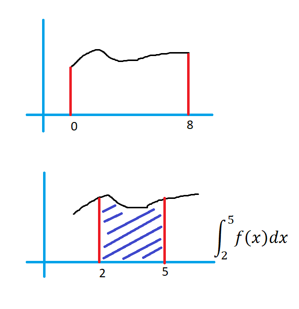
Assume, the function y = f(x)

The function y = f(x) exist from x = 0 to x =8.

The above diagram shows the shape of the function.

Taking the integral of f(x) from 2 to 5 will give the area under the function f(x).

Now we refresh discrete probability distribution and then go with continuous.

The below diagram shows the discrete probability distribution for the random variable X = 0, 1, 2, 3, 4, 5.

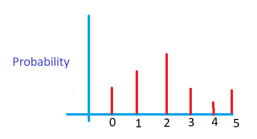
X in range 0 – 5.

The discrete probability distribution takes a few values present in the range.

The conditions satisfied by discrete probability functions is the sum of all probability values = 1

1) for all x Σ f(x) = 1

2) for all x f(x) >= 0

The function which satisfies the above two conditions is the discrete probability function.

Continuous Probability Distribution

Take a continuous random variable X.

The variable X ranges from 0 -5.

In continuous probability distribution, X can take any value in the range 0 – 5

X can take 0, 0.1, 0.01, . . 5

The below diagram shows the function f(x).

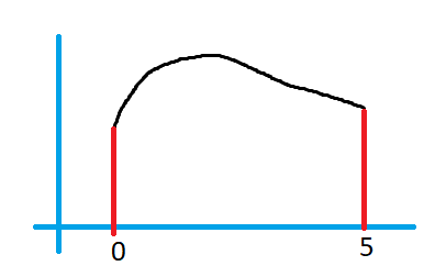
The distribution of the probabilities of random variable X is as explained below.

The function f(x) should satisfy the below conditions.

1) Integral of f(x) from 0-1 should equal 1.

From the first condition, the area under the function should be 1.

We distribute the probabilities in the area under the function.

2) integral of f(x) values should be always >=0.

The below diagram shows the area under the integral value.

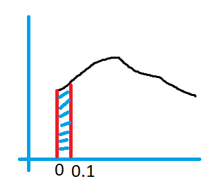
The integral value obtained is the probability value because of the distribution of probabilities under the area.

Functions that satisfy the above two conditions are probability Density Functions.