Mode for Frequency Distributions

In this class, We discuss Mode for Frequency Distributions.

For Complete YouTube Video: Click Here

The reader should have prior knowledge of the mode. Click Here.

Example 1: Discrete Values

The below table shows the frequency distribution of shirts data.

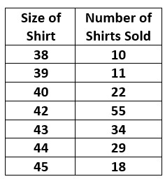
The table shows the size of the shirts and the number of shirts sold.

Mode = the shirt having the highest frequency = 42 sizes has frequency value 55.

Mode for continuous values:

The below table shows the continuous frequency distribution.

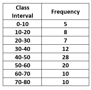
The class with the highest frequency value is considered the mode class.

Fm = mode class

The interval of the model class is 40 – 50.

Giving a mode value of 40 is not good because the left side will have less number of data values.

Giving a mode value of 50 is not good because the right side will have less number of data values.

We discussed a similar logic in the median class. Click Here.

The measure of central tendency should always go with the central value, and we need to find a value between 40 and 50.

F0 = frequency of the class before mode class.

F2 = frequency of the class after mode class.

Mode = L + h((Fm – F0)/((Fm – F0) + (Fm – F2)).

L is the lower limit of the modal class.

‘h’ is the length of interval for modal class.

Based on the frequencies of previous and after classes, the equation will assign a value between the modal class interval.

Substituting the values we get mode = 40 + 10(16/24)

Mode = 46.67