Distance Vector Routing Algorithm 3

For Complete YouTube Video: Click Here

In this class, we will try to understand Distance Vector Routing Algorithm 3.

We have already discussed the main parts of the distance vector routing in our previous classes.

Distance Vector Routing Algorithm 3

In competitive exams like GATE, IES, and Semester end exams, we can solve the questions asked on distance vector routing after generating the routing tables.

We don’t need to follow all the steps to get the final routing table in those exams.

Just by using our intuition, we can generate the routing tables.

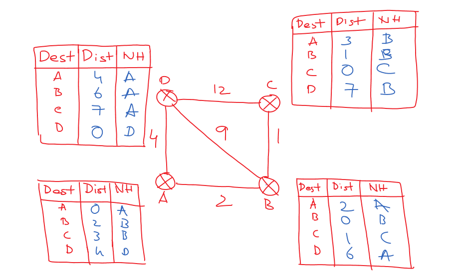
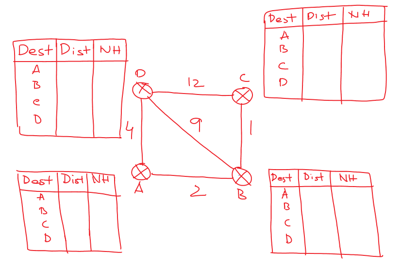
For understanding, we will consider the sample network shown below.

In the above network, we can see that the shortest distance from A -> B is 2, which is directly from A -> B.

We have many other paths like A -> D -> B with a distance of 13, and another approach is from A-> D -> C -> B with a distance of 17.

With this simple intuition, we generate the final routing tables in less time.

The image below shows the final output.